This paper (Liu et al. 2024) proposes an alternative to multi-layer
perceptrons (MLPs) in machine learning.
The basic idea is that MLPs have parameters on the nodes of the
computation graph (the weights and biases on each cell), and that KANs
have the parameters on the edges. Each edge has a learnable activation
function parameterized as a spline.
The network is learned at two levels, which allows for “adjusting
locally”:
the overall shape of the computation graph and its connexions
(external degrees of freedom, to learn the compositional structure),
the parameters of each activation function (internal degrees of
freedom).
It is based on the Kolmogorov-Arnold representation theorem, which
says that any continuous multivariate function can be represented as a
sum of continuous univariate functions. We recover the distinction
between the compositional structure of the sum and the structure of
each internal univariate function.
The theorem can be interpreted as two layers, and the paper then
generalizes it to multiple layer of arbitrary width. In the theorem,
the univariate functions are arbitrary and can be complex (even
fractal), so the hope is that allowing for arbitrary depth and width
will allow to only use splines. They derive an approximation theorem:
when replacing the arbitrary continuous functions of the
Kolmogorov-Arnold representation with splines, we can bound the error
independently of the dimension. (However there is a constant which
depends on the function and its representation, and therefore on the
dimension…) Theoretical scaling laws in the number of parameters are
much better than for MLPs, and moreover, experiments show that KANs
are much closer to their theoretical bounds than MLPs.
KANs have interesting properties:
The splines are interpolated on grid points which can be iteratively
refined. The fact that there is a notion of “fine-grainedness” is
very interesting, it allows to add parameters without having to
retrain everything.
Larger is not always better: the quality of the reconstruction
depends on finding the optimal shape of the network, which should
match the structure of the function we want to approximate. Finding
this optimal shape is found via sparsification, pruning, and
regularization (non-trivial).
We can have a “human in the loop” during training, guiding pruning,
and “symbolifying” some activations (i.e. by recognizing that an
activation function is actually a cos function, replace it
directly). This symbolic discovery can be guided by a symbolic
system recognizing some functions. It’s therefore a mix of symbolic
regression and numerical regression.
They test mostly with scientific applications in mind: reconstructing
equations from physics and pure maths. Conceptually, it has a lot of
overlap with Neural Differential Equations
(Chen et al. 2018; Ruthotto 2024)
and “scientific ML” in general.
There is an interesting discussion at the end about KANs as the model
of choice for the “language of science”. The idea is that LLMs are
important because they are useful for natural language, and KANs
could fill the same role for the language of functions. The
interpretability and adaptability (being able to be manipulated and
guided during training by a domain expert) is thus a core feature that
traditional deep learning models lack.
There are still challenges, mostly it’s unclear how it performs on
other types of data and other modalities, but it is very
encouraging. There is also a computational challenges, they are
obviously much slower to train, but there has been almost no
engineering work on them to optimize this, so it’s expected. The fact
that the operations are not easily batchable (compared to matrix
multiplication) is however worrying for scalability to large networks.
References
Chen, Ricky T. Q., Yulia Rubanova, Jesse Bettencourt, and David Duvenaud. 2018. “Neural Ordinary Differential Equations,” June. http://arxiv.org/abs/1806.07366.
Liu, Ziming, Yixuan Wang, Sachin Vaidya, Fabian Ruehle, James Halverson, Marin Soljačić, Thomas Y. Hou, and Max Tegmark. 2024. “KAN: Kolmogorov-ArnoldNetworks.” arXiv. https://doi.org/10.48550/arXiv.2404.19756.
Ruthotto, Lars. 2024. “Differential Equations for Continuous-TimeDeepLearning.”Notices of the American Mathematical Society 71 (05). https://doi.org/10.1090/noti2930.
]]>Randomness and Uncertainty: from random noise to predictable oscillations via differential equationshttps://www.lozeve.com/posts/randomness-and-uncertainty.html2023-10-20T00:00:00Z2023-10-20T00:00:00Z
There are many ways to generate pseudo-random numbers that look
perfectly “random” but are actually the output of fully deterministic
processes. Trefethen gives an example of a chaotic system based on a
logistic equation.
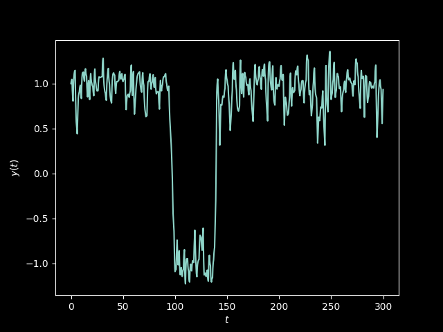
But more interesting (to me) and more original may be the other way
around: how to get certainty from randomness. There are ordinary
differential equations that can take random noise as input, and whose
solution is very stable, oscillating between two possible
values. Given a function \(f\) approximating random white noise, the
solution to the ODE
\[ y' = y - y^3 + Cf(t) \]
is “bistable” and remains always around -1 and 1. The parameter \(C\)
allows to control the half-life of the transitions.
To explore this behaviour, I replicated Trefethen’s experiments in
Python with the Diffrax library (a differential equations solver based
on JAX). The full code is in this Gist.
It suffices to define a simple function for the vector field and to
give it to a solver:
def f(t, y, args):return y - y**3+0.4* args[t.astype(int)]
where args will be the input, as a simple array of
normally-distributed random values. \(C\) is hardcoded as 0.4 as in the
article, but could be passed through args as well (it can be a
dictionary).
Dietterich (2018) is an
interesting article about how to make robust AI. High risk
situations require the combined AI and human system to operate as a
high reliability organization (HRO). Only such an organization can
have sufficiently strong safety and reliability properties to ensure
that powerful AI systems will not amplify human mistakes.
Reliability and high-reliability organizations
The concept of high reliability organization (HRO) comes from
Weick, Sutcliffe, and Obstfeld (1999). Examples of HROs include nuclear power
plants, aircraft carriers, air traffic control systems, and space
shuttles. They share several characteristics: an unforgiving
environment, vast potential for error, and dramatic scales in the case
of a failure.
The paper identifies five processes common to HROs, that they group
into the concept of mindfulness (a kind of “enriched
awareness”). Mindfulness is about allocating and conserving attention
of the group. It includes both being consciously aware of the
situation and acting on this understanding.
This mindfulness leads to the capacity to discover and manage
unexpected events, which in turn leads to reliability.
Characteristics of a high reliability organization
An HRO is an organization with the following five attributes.
Preoccupation with failure
Failures in HROs are extremely rare. To make it easier to learn from
them, the organization has to broaden the data set by expanding the
definition of failure and studying all types of anomalies and near
misses. Additionally, the analysis is much richer, and always
considers the reliability of the entire system, even for localized
failures.
HROS also study the absence of failure: why it didn’t fail, and the
possibility that no flaws were identified because there wasn’t enough
attention to potential flaws.
To further increase the number of data point to study, HROs encourage
reporting all mistakes and anomalies by anyone. Contrary to most
organizations, members are rewarded for reporting potential failures,
even if their analysis is wrong or if they are responsible for
them. This creates an atmosphere of “psychological safety” essential
for transparency and honesty in anomaly reporting.
Reluctance to simplify interpretations
HROs avoid having a single interpretation for a given event. They
encourage generating multiple, complex, contradicting interpretations
for every phenomenon. These varied interpretations enlarge the number
of concurrent precautions. Redundancy is implemented not only via
duplication, but via skepticism of existing systems.
People are encouraged to have different views, different backgrounds,
and are re-trained often. To resolve the contradictions and the
oppositions of views, interpersonal and human skills are highly
valued, possibly more than technical skills.
Sensitivity to operations
HROs rely a lot on “situational awareness”. They are ensuring that no
emergent phenomena emerge in the system: all outputs should always be
explained by the known inputs. Otherwise, there might be other forces
at work that need to be identified and dealt with. A small group of
people may be dedicated to this awareness at all times.
Commitments to resilience
HROs train people to be experts at combining all processes and events
to improve their reactions and their improvisation skills. Everyone
should be an expert at anticipating potential adverse events, and
managing surprise. When events get outside normal operational
boundaries, organizations members self-organize into small dedicated
teams to improvise solutions to novel problems.
Underspecification of structures
There is no fixed reporting path, anyone can raise an alarm and halt
operations. Everyone can take decisions related to their technical
expertise. Information is spread directly through the organization, so
that people with the right expertise are warned first. Power is
delegated to operation personal, but management is completely
available at all times.
HROs vs non-HROs
Non-HROs increasingly exhibit some properties of HROs. This may be due
to the fact that highly competitive environments with short cycles
create unforgiving conditions (high performance standards, low
tolerance for errors). However, most everyday organizations do not put
failure at the heart of their thinking.
Failures in non-HROs come from the same sources: cultural assumptions
on the effectiveness or accuracy of previous precautions measures.
Preoccupation with failure also reveal the couplings and the complex
interactions in the manipulated systems. This in turn leads to
uncoupling and less emergent behaviour over time. People understand
better long-term, complex interactions.
Reliability vs performance, and the importance of learning
An interesting discussion is around the (alleged) trade-off between
reliability and performance. It is assumed that HROs put the focus on
reliability at the cost of throughput. As a consequence, it may not
make sense for ordinary organizations to put as much emphasis on
safety and reliability, as the cost to the business may be
prohibitive.
However, investments in safety can also be viewed as investments in
learning. HROs view safety and reliability as a process of search
and learning (constant search for anomalies, learning the interactions
between the parts of a complex system, ensuring we can link outputs to
known inputs). As such, investments in safety encourage collective
knowledge production and dissemination.
Mindfulness also stimulates intrinsic motivation and perceptions of
efficacy and control, which increase individual performance. (People
who strongly believe they are in control of their own output are more
motivated and more efficient.)
HROs may encourage mindfulness based on operational necessity in front
of the catastrophic consequences of any failure, but non-HROs can
adopt the same practice to boost efficiency and learning to gain
competitive advantage.
Additional lessons that can be learned from HROs (implicit in the
previous discussion):
The expectation of surprise is an organizational resource because
it promotes real-time attentiveness and discovery.
Anomalous events should be treated as outcomes rather than
accidents, to encourage search for sources and causes.
Errors should be made as conspicuous as possible to undermine
self-deception and concealment.
Reliability requires diversity, duplication, overlap, and a varied
response repertoire, whereas efficiency requires homogeneity,
specialization, non-redundancy, and standardization.
Interpersonal skills are just as important in HROs as are technical
skills.
References
Dietterich, Thomas G. 2018. “Robust Artificial Intelligence and Robust Human Organizations.”CoRR. http://arxiv.org/abs/1811.10840.
Weick, Karl E., Kathleen M. Sutcliffe, and David Obstfeld. 1999. “Organizing for High Reliability: Processes of Collective Mindfulness.” In Research in Organizational Behavior, edited by R. S. Sutton and B. M. Staw, 21:81–123. Research in Organizational Behavior, Vol. 21. Stanford: Elsevier Science/JAI Press. https://archive.org/details/organizing-for-high-reliability.
]]>How to train your differentiable filterhttps://www.lozeve.com/posts/how-to-train-your-differentiable-filter.html2022-05-20T00:00:00Z2022-05-20T00:00:00Z
This is a short overview of the following paper (Kloss, Martius, and Bohg 2021):
Kloss, Alina, Georg Martius, and Jeannette Bohg. 2021. “How to Train
Your Differentiable Filter.” Autonomous Robots 45 (4):
561–78. https://doi.org/10.1007/s10514-021-09990-9.
Bayesian filtering for state estimation
Bayesian filters(Thrun 2006) contains a
great explanation of Bayesian filters (including Kalman and particle
filters), in the context of robotics, which is relevant for this
paper. For a more complete overview of Kalman filters, see
(Anderson and Moore 2005).
are the standard method for
probabilistic state estimation. Common examples are (extended,
unscented) Kalman filters and particle filters. These filters require
a process model predicting how the state evolves over time, and an
observation model relating an sensor value to the underlying state.
The objective of a filter for state estimation is to estimate a latent
state \(\mathbf{x}\) of a dynamical system at any time step \(t\) given an
initial belief \(\mathrm{bel}(\mathbf{x}_0) = p(\mathbf{x}_0)\), a
sequence of observations \(\mathbf{z}_{1\ldots t}\), and controls
\(\mathbf{u}_{0\ldots t}\).
We make the Markov assumption (i.e. states and observations are
conditionally independent from the history of past states).
where \(\eta\) is a normalization factor. Computing
\(\overline{\mathrm{bel}}(\mathbf{x}_t)\) is the prediction step, and
applying \(p(\mathbf{z}_t | \mathbf{x}_t)\) is the update step (or the
observation step).
We model the dynamics of the system through a process model \(f\) and an
observation model \(h\):
\[
\begin{align*}
\mathbf{x}_t &= f(\mathbf{x}_{t-1}, \mathbf{u}_{t-1}, \mathbf{q}_{t-1})\\
\mathbf{z}_t &= h(\mathbf{x}_t, \mathbf{r}_t),
\end{align*}
\]
where \(\mathbf{q}\) and \(\mathbf{r}\) are random variables representing
process and observation noise, respectively.
Differentiable Bayesian filters
These models are often difficult to formulate and specify, especially
when the application has complex dynamics, with complicated noises,
nonlinearities, high-dimensional state or observations, etc.
To improve this situation, the key idea is to learn these complex
dynamics and noise models from data. Instead of spending hours in
front of a blackboard deriving the equations, we could give a simple
model a lot of data and learn the equations from them!
In the case of Bayesian filters, we have to define the process,
observation, and noise processes as parameterized functions
(e.g. neural networks), and learn their parameters end-to-end, through
the entire apparatus of the filter. To learn these parameters, we will
use the simplest method: gradient descent. Our filter have to become
differentiable.
The paper shows that such differentiable filters (trained
end-to-end) outperform unstructured LSTMs, and outperform standard
filters where the process and observation models are fixed in advance
(i.e. analytically derived or even trained separately in isolation).
In most applications, the process and observation noises are often
assumed to be uncorrelated Gaussians, with zero mean and constant
covariance (which is a hyperparameter of the filter). With end-to-end
training, we can learn these parameters (mean and covariance of the
noise), but we can even go further, and use heteroscedastic noise
models. In this model, the noise can depend on the state of the system
and the applied control.
Learnable process and observation models
The observation model \(f\) can be implemented as a simple feed-forward
neural network. Importantly, this NN is trained to output the
difference between the next and the current state (\(\mathbf{x}_{t+1} - \mathbf{x}_t\)).
This ensure stable gradients and an easier initialization near the
identity.
For the observation model, we could do the same and model \(g\) as a
generative neural network predicting the output of the
sensors. However, the observation space is often high-dimensional, and
the network is thus difficult to train. Consequently, the authors use
a discriminative neural network to reduce the dimensionality of the
raw sensory output.
Learnable noise models
In the Gaussian case, we use neural networks to predict the covariance
matrix of the noise processes. To ensure positive-definiteness, the
network predicts an upper-triangular matrix \(\mathbf{L}_t\) and the
noise covariance matrix is set to \(\mathbf{Q}_t = \mathbf{L}_t \mathbf{L}_t^T\).
In the heteroscedastic case, the noise covariance is predicted from
the state and the control input.
Loss function
We assume that we have access to the ground-truth trajectory \(\mathbf{x}_{1\ldots T}\).
We can then use the mean squared error (MSE) between the ground truth
and the mean of the belief:
Alternatively, we can compute the negative log-likelihood of the true
state under the belief distribution (represented by a Gaussian of mean
\(\mathbf{\mu}_t\) and covariance \(\mathbf{\Sigma}_t\)):
Some are easy because they use only differentiable operations (mostly
simple linear algebra). For the EKF, we also need to compute
Jacobians. This can be done automatically via automatic
differentiation, but the authors have encountered technical
difficulties with this (memory consumption or slow computations), so
they recommend computing Jacobians manually.It is not clear
whether this is a limitation of automatic differentiation, or of their
specific implementation with TensorFlow. Some other projects have
successfully computed Jacobians for EKFs with autodiff libraries, like
GaussianFilters.jl in Julia.
The particle filter has a resampling step that is not differentiable:
the gradient cannot be propagated to particles that are not selected
by the sampling step. There are apparently specific resampling
algorithms that help mitigate this issue in practice when training.
Conclusions
Differentiable filters achieve better results with fewer parameters
than unstructured models like LSTMs, especially on complex tasks. The
paper runs extensive experiments on various toy models of various
complexity, although unfortunately no real-world application is shown.
Noise models with full covariance improve the tracking
accuracy. Heteroscedastic noise models improve it even more.
The main issue is to keep the training stable. They recommend the
differentiable extended Kalman filter for getting started, as it is
the most simple filter, and is less sensitive to hyperparameter
choices. If the task is strongly non-linear, one should use a
differentiable unscented Kalman filter or a differentiable particle
filter.
References
Anderson, Brian D. O., and John B. Moore. 2005. Optimal Filtering. Dover Books on Electrical Engineering. Dover Publications.
Kloss, Alina, Georg Martius, and Jeannette Bohg. 2021. “How to Train Your Differentiable Filter.”Autonomous Robots 45 (4): 561–78. https://doi.org/10.1007/s10514-021-09990-9.
]]>The Dawning of the Age of Stochasticityhttps://www.lozeve.com/posts/dawning-of-the-age-of-stochasticity.html2022-03-24T00:00:00Z2022-03-24T00:00:00Z
Mumford, David. 2000. “The Dawning of the Age of Stochasticity.”
Atti Della Accademia Nazionale Dei Lincei. Classe Di Scienze Fisiche,
Matematiche E Naturali. Rendiconti Lincei. Matematica E Applicazioni
11: 107–25. http://eudml.org/doc/289648.
This article (Mumford 2000) is an interesting call
for a new set of foundations of mathematics on probability and
statistics. It argues that logic has had its time, and now we should
make random variables a first-class concept, as they would make for
better foundations.
The taxonomy of mathematics
This is probably the best definition of mathematics I have
seen. Before that, the most satisfying definition was “mathematics is
what mathematicians do”. It also raises an interesting question: what
would the study of non-reproducible mental objects be?
The study of mental objects with reproducible properties is called mathematics.
(Davis, Hersh, and Marchisotto 2012)
What are the categories of reproducible mental objects? Mumford
considers the principal sub-fields of mathematics (geometry, analysis,
algebra, logic) and argues that they are indeed rooted in common
mental phenomena.
Of these, logic, and the notion of proposition, with an absolute truth
value attached to it, was made the foundation of all the
others. Mumford’s argument is that instead, the random variable is (or
should be) the “paradigmatic mental object”, on which all others can
be based. People are constantly weighing likelihoods, evaluating
plausibility, and sampling from posterior distributions to refine
estimates.
As such, random variables are rooted in our inspection of our own
mental processes, in the self-conscious analysis of our minds. Compare
to areas of mathematics arising from our experience with the physical
world, through our perception of space (geometry), of forces and
accelerations (analysis), or through composition of actions (algebra).
The paper then proceeds to do a quick historical overview of the
principal notions of probability, which mostly mirror the detailed
historical perspective in (Hacking 2006). There is
also a short summary of the work into the foundations of mathematics.
Mumford also claims that although there were many advances in the
foundation of probability (e.g. Galton, Gibbs for statistical physics,
Keynes in economics, Wiener for control theory, Shannon for
information theory), most important statisticians (R. A. Fisher)
insisted on keeping the scope of statistics fairly limited to
empirical data: the so-called “frequentist” school. (This is a vision
of the whole frequentist vs Bayesian debate that I hadn’t seen
before. The Bayesian school can be seen as the one who claims that
statistical inference can be applied more widely, even to real-life
complex situations and thought processes. In this point of view, the
emergence of the probabilistic method in various areas of science
would be the strongest argument in favour of bayesianism.)
What is a “random variable”?
Random variables are difficult to define. They are the core concept of
any course in probability of statistics, but their full, rigorous
definition relies on advanced measure theory, often unapproachable to
beginners. Nevertheless, practitioners tend to be productive with
basic introductions to probability and statistics, even without
being able to formulate the explicit definition.
Here, Mumford discusses the various definitions we can apply to the
notion of random variable, from an intuitive and a formal point of
view. The conclusion is essentially that a random variable is a
complex entity that do not easily accept a satisfying definition,
except from a purely formal and axiomatic point of view.
This situation is very similar to the one for the notion of
“set”. Everybody can manipulate them on an intuitive level and grasp
the basic properties, but the specific axioms are hard to grasp, and
no definition is fully satisfying, as the debates on the foundations
of mathematics can attest.
Putting random variables into the foundations
The usual way of defining random variables is:
predicate logic,
sets,
natural numbers,
real numbers,
measures,
random variables.
Instead, we could put random variables at the foundations, and define
everything else in terms of that.
There is no complete formulation of such a foundation, nor is it clear
that it is possible. However, to make his case, Mumford presents two
developments. One is from E. T. Jaynes, who has a complete formalism
of Bayesian probability from a notion of “plausibility”. With a few
axioms, we can obtain an isomorphism between an intuitive notion of
plausibility and a true probability function.
The other example is a proof that the continuum hypothesis is false,
using a probabilistic argument, due to Christopher Freiling. This
proof starts from a notion of random variable that is incompatible
with the usual definition in terms of measure theory. However, this
leads Mumford to question whether a foundation of mathematics based on
such a notion could get us rid of “one of the meaningless conundrums
of set theory”.
Stochastic methods have invaded classical mathematics
This is probably the most convincing argument to give a greater
importance to probability and statistical methods in the foundations
of mathematics: there tend to be everywhere, and extremely
productive. A prime example is obviously graph theory, where the
“probabilistic method” has had a deep impact, thanks notably to
Erdős. (See (Alon and Spencer 2016) and Timothy Gowers’ lessons at the Collège de FranceIn French, but see also his YouTube channel.
on the probabilistic method for combinatorics and number
theory.) Probabilistic methods also have a huge importance in the
analysis of differential equations, chaos theory, and mathematical
physics in general.
Thinking as Bayesian inference
I think this is not very controversial in cognitive science: we do not
think by composing propositions into syllogisms, but rather by
inferring probabilities of certain statements being true. Mumford
illustrates this very well with an example from Judea Pearl, which
uses graphical models to represent thought processes. There is also a
link with formal definitions of induction, such as PAC learning, which
is very present in machine learning.
I’ll conclude this post by quoting directly the last paragraph of the
article:
My overall conclusion is that I believe stochastic methods will
transform pure and applied mathematics in the beginning of the third
millennium. Probability and statistics will come to be viewed as the
natural tools to use in mathematical as well as scientific modeling.
The intellectual world as a whole will come to view logic as a
beautiful elegant idealization but to view statistics as the standard
way in which we reason and think.
References
Alon, Noga, and Joel H. Spencer. 2016. The Probabilistic Method. 4th ed. Wiley.
Davis, Philip J., Reuben Hersh, and Elena Anne Marchisotto. 2012. The Mathematical Experience, Study Edition. Modern Birkhäuser Classics. Birkhäuser Boston. https://doi.org/10.1007/978-0-8176-8295-8.
Hacking, Ian. 2006. The Emergence of Probability: A Philosophical Study of Early Ideas about Probability, Induction and Statistical Inference. 2nd ed. Cambridge University Press. https://doi.org/10.1017/CBO9780511817557.
Mumford, David. 2000. “The Dawning of the Age of Stochasticity.”Atti Della Accademia Nazionale Dei Lincei. Classe Di Scienze Fisiche, Matematiche e Naturali. Rendiconti Lincei. Matematica e Applicazioni 11 (December): 107–25. http://eudml.org/doc/289648.
]]>Planning and scheduling for project managementhttps://www.lozeve.com/posts/planning-and-scheduling.html2021-04-13T00:00:00Z2021-04-13T00:00:00Z
Every project, no matter its size, requires some kind of organization
and planning. Whether you’re thinking about what you need to do when
you wake up (shower, make breakfast, brush your teeth) or planning a
new space programme, you will need to think about the tasks, in what
order to do them, and how long it will take. This is called
scheduling.
Planning projects requires balancing dependencies between tasks,
resource allocation, and complex constraints in order to find a
complete and feasible schedule. How much of this can be made rigorous?
What is the limit of automation in this scenario?
In this post, I want to explore the problem of planning and scheduling
in the specific context of project management. The goal is to set up
the problem of project planning rigorously, and investigate what
techniques we can apply to have a better understanding of our projects
and reach our objectives faster.
General project management workflow
When starting a new projectThe definition of a project here is highly subjective,
and has been strongly influenced by what I’ve read (see the
references) and how I actually do things at work. In particular, most
of the model and concepts can be found in Microsoft Project.
, I generally follow a rough
workflow that goes like this:
Define the global constraints of the project: functional
specification, deadlines, overall resources available, etc.
Subdivide the projects into tasks and subtasks. Low-level tasks
should be self-contained and doable by few people (ideally only
one). Tasks can then be grouped together for better visualising
what is happening at various scales. This gives us a global
hierarchy of tasks, culminating in the overall project.
Specify the dependencies between tasks, ideally with an explicit
deliverable for each dependency relationship.
Estimate the work required for each task.
Affect a resource to each task, deriving task durations
accordingly. For instance, if Bob will be working part-time on this
task (because he has other things to do at the same time), the task
will take longer to complete than the nominal amount of work that
it requires.
Find an order in which to execute all the tasks, respecting
workforce and time constraints (Bob cannot spend 50% of this time
on three tasks simultaneously). This is called a schedule.
Iterate on the order until a minimal completion date is
found. Generally, the objective is to complete the project as soon
as possible, but there may be additional requirements (overall
deadline, lateness penalties, maximal resource utilization).
Given this process, a natural question would be to ask: how can we
simplify it? What can we automate? The obvious task is the scheduling
part (steps 6 and 7): this step does not require any human
decision-making, and for which it will be difficult and tiresome to
achieve optimality. Most project management software (e.g. Microsoft Project) focus on this part.
However, in practice, resource allocation is also extremely time
consuming. Most importantly, it will constrain the final schedule: a
bad allocation can push back the final completion date by a wide
margin. Therefore, it makes sense to want to take into account both
resource allocation and task ordering at the same time when looking
for an optimal schedule.
Going even further, we could look into subdividing tasks further:
maybe splitting a task in two, allowing a small lag between the
completion of the first half and the start of the second half, could
improve the overall objective. By allowing preemption, we could
optimize further our schedule.
To understand all of this, we’ll need to formalize our problem a
little bit. This will allow us to position it in the overall schema of
problems studied in the operations research literature, and use their
conclusions to choose the best approach as a trade-off between manual
and automatic scheduling.
The project scheduling problem
A project is simply a set of tasksA task is often called a job or an activity in project
scheduling. I will use these terms interchangeably.
. Each
task is a specific action with a certain amount of work that needs to
be done. More importantly, a task can depend on other tasks: for
instance, I can’t send the satellite in the space if you haven’t built
it yet.
Other constraints may also be present: there are nearly always
deadlines (my satellite needs to be up and running on 2024-05-12), and
sometimes other kind of temporal constraints (for legal reasons, I
can’t start building my death ray before 2023-01-01). Most
importantly, there are constraints on resource usage (I need either
Alice or Bob to work on these tasks, so I will be able to work on at
most two of them at the same time).
Finally, the objective is to finish the project (i.e. complete all
the tasks) as early as possible. This is called the makespan.
You may have noticed a nice pattern here: objective, constraints? We
have a great optimization problem! As it turns out, scheduling is an
entire branch of operations researchSee my previous blog post on operations research.
. In the
literature, this kind of problem is referred to as
resource-constrained project scheduling, or as project scheduling
with workforce constraints.
Classification of scheduling problems
There is a lot of room to modify the problem to other settings.
Brucker et al. (1999) propose an interesting
classification scheme for project scheduling. In this system, any
problem can be represented by a triplet \(\alpha|\beta|\gamma\), where
\(\alpha\) is the resource environment, \(\beta\) are the activity
characteristics, and \(\gamma\) is the objective function.
The resource environment\(\alpha\) describes the available quantity
of each type of resources. Resource can be renewable, like people, who
supply a fixed quantity of work in each time period, or non-renewable,
like raw materials.
The activity characteristics\(\beta\) describe how tasks are
constrained: how the dependencies are specified (with a graph, or with
temporal constraints between the starts and ends of different tasks),
whether there are global constraints like deadlines, and whether
processing times are constant for all tasks, can vary, or even can be
stochastic.
Finally, the objective\(\gamma\) can be one of several
possibilities. The most common are the makespan which seeks to
minimize the total duration of the project, and resource-levelling
which seeks to minimize some measure of variation of resource
utilization.
Some important problems (\(\mathrm{PS}\) means “project scheduling”
without any restrictions on resources):
\(\mathrm{PS} \;|\; \mathrm{prec} \;|\; C_{\max}\): the “simple”
project scheduling setup, which corresponds to the practical
application that interests us here. Although this is the base
problem, it is still quite challenging. Removing the resource
constraints renders the problem much easier from a computational
point of view (Pinedo 2009, chap. 4).
\(\mathrm{PS} \;|\; \mathrm{temp} \;|\; C_{\max}\): when you add time
lag constraints (e.g. two tasks that must start within two days of
each other), the problem becomes much more difficult.
\(\mathrm{PS} \;|\; \mathrm{temp} \;| \sum c_{k} f\left(r_{k}(S,
t)\right)\): this is the resource-levelling problem: you want to
minimize the costs of using an amount \(r_k(S, t)\) of each resource
\(k\), when each unit of resource costs \(c_k\).
Algorithms for project scheduling
Without workforce constraints
First, we need a way to represent a project. We can use the so-called
job-on-node formatThere is also a job-on-arc format that is apparently
widely used, but less practical in most applications.
. The nodes represent the tasks in
the precedence graph, and arcs represent the dependency relationships
between tasks.
This representation leads to a natural algorithm for project
scheduling in the absence of any resource constraints. The critical path method (CPM) consists in finding a chain of dependent tasks in
the job-on-node graph that are critical: their completion time is
fixed by their dependencies.
It consists of two procedures, one to determine the earliest possible
completion time of each task (forward procedure), and one to determine
the latest possible completion time of each task that does not
increase total project duration (backward procedure). The tasks for
which these two times are equal form the critical
pathNote that the critical path is not necessarily
unique, and several critical paths may be overlapping.
. Non-critical tasks have a certain amount of
slack: it is possible to schedule them freely between the two
extremities without affecting the makespan.
An extension of the critical path method is the program evaluation and review technique (PERT). We still consider we have unlimited
resources, but the processing time of each task is allowed to be a
random variable instead of a fixed quantity. The algorithm must be
amended correspondingly to take into account pessimistic and
optimistic estimates of each task duration.
These techniques have been widely employed in various
industriesWikipedia tells us that CPM and PERT were partly
developed by the US Navy, and applied to several large-scale projects,
like skyscraper buildings, aerospace and military projects, the
Manhattan project, etc.
, and show that the project scheduling
problem without workforce constraints can be solved extremely
efficiently. See Pinedo (2009) for more
details on these algorithms and some examples.
With workforce constraints
With resource constraints, the problem becomes much harder to
solve. It is not possible to formulate this problem as a linear
program: workforce constraints are intrinsically combinatorial in
nature, so the problem is formulated as an integer
programThe full integer program can be found in
Pinedo (2009, sec. 4.6).
.
The problem is modelled with 0-1 variables \(x_{jt}\) which take the
value 1 if job \(j\) is completed exactly at time \(t\), and 0
otherwise. The objective is to minimize the makespan, i.e. the
completion time of a dummy job that depends on all other jobs. There
are three constraints:
if job \(j\) is a dependency of job \(k\), the completion time of job
\(k\) is larger than the completion time of job \(j\) plus the duration
of job \(k\),
at any given time, we do not exceed the total amount of resources
available for each type of resources,
all jobs are completed at the end of the project.
This problem quickly becomes challenging from a computational point of
view when the number of tasks increase. Variations on the branch and bound method have been developed to solve the resource-constrained
project scheduling problem efficiently, and in practice most
applications rely on heuristics to approximate the full
problem. However, even special cases may be extremely challenging to
solve. The project scheduling problem is a generalization of the job shop scheduling problem, which is itself a generalization of the
travelling salesman problem: all of these are therefore NP-hard.
See Brucker et al. (1999) for a short survey of
algorithms and heuristics, and extensions to the harder problems
(multi-mode case, time-cost trade-offs, other objective
functions). Pinedo (2016) contains a much more extensive
discussion of all kinds of scheduling problems, algorithms, and
implementation considerations.
Further reading
Brucker et al. (1999) is a great survey of the
algorithms available for project scheduling. For longer books,
Pinedo (2016), Brucker (2007),
Conway, Maxwell, and Miller (2003), and Leung (2004) are good
references for the theoretical aspects, and
Pinedo (2009) and
Błażewicz et al. (2001) for applications.
Atabakhsh (1991),
Noronha and Sarma (1991), and
Smith (1992) contain
algorithms that use methods from artificial intelligence to complement
the traditional operations research approach.
Automating project management
Let us review our workflow from the beginning. Even for the general
case of project scheduling with workforce and temporal constraints,
algorithms exist that are able to automate the entire scheduling
problem (except maybe for the largest projects). Additional
manipulations can easily be encoded with these two types of
constraints.
Most tools today seem to rely on a variant of CPM or
PERTThis seems to be the case for Microsoft Project at
least. However, I should note that it is an enormous piece of
software, and I barely scratched the surface of its capabilities. In
particular, it can do much more that project scheduling: there are
options for resource levelling and budgeting, along with a lot of
visualization and reporting features (Gantt charts).
. As a result, you still have to manually allocate
resources, which can be really time-consuming on large projects:
ensuring that each resource is not over-allocated, and finding which
task to reschedule while minimizing the impact on the overall project
duration is not obvious at all.
As a result, a tool that would allow me to choose the level of control
I want in resource allocation would be ideal. I could explicitly set
the resources used by some tasks, and add some global limits on which
resources are available for the overall project, and the algorithm
would do the rest.
We could then focus on automating further, allowing preemption of
tasks, time-cost trade-offs, etc. Finding the right abstractions and
selecting the best algorithm for each case would be a challenging
project, but I think it would be extremely interesting!
References
Atabakhsh, H. 1991. “A Survey of Constraint Based Scheduling Systems Using an Artificial Intelligence Approach.”Artificial Intelligence in Engineering 6 (2): 58–73. https://doi.org/10.1016/0954-1810(91)90001-5.
Błażewicz, Jacek, Klaus H. Ecker, Erwin Pesch, Günter Schmidt, and Jan Węglarz. 2001. Scheduling Computer and Manufacturing Processes. 2nd ed. Springer Berlin Heidelberg. https://doi.org/10.1007/978-3-662-04363-9.
Brucker, Peter, Andreas Drexl, Rolf Möhring, Klaus Neumann, and Erwin Pesch. 1999. “Resource-Constrained Project Scheduling: Notation, Classification, Models, and Methods.”European Journal of Operational Research 112 (1): 3–41. https://doi.org/10.1016/s0377-2217(98)00204-5.
Conway, Richard, William L. Maxwell, and Louis W. Miller. 2003. Theory of Scheduling. Mineola, N.Y: Dover.
Leung, Joseph. 2004. Handbook of Scheduling : Algorithms, Models, and Performance Analysis. Boca Raton: Chapman & Hall/CRC.
Noronha, S. J., and V. V. S. Sarma. 1991. “Knowledge-Based Approaches for Scheduling Problems: A Survey.”IEEE Transactions on Knowledge and Data Engineering 3 (2): 160–71. https://doi.org/10.1109/69.87996.
Pinedo, Michael L. 2009. Planning and Scheduling in Manufacturing and Services. 2nd ed. Springer Series in Operations Research and Financial Engineering. New York: Springer. https://doi.org/10.1007/978-1-4419-0910-7.
Smith, Stephen F. 1992. “Knowledge-Based Production Management Approaches, Results and Prospects.”Production Planning & Control 3 (4): 350–80. https://doi.org/10.1080/09537289208919407.
]]>Solving a problem with mathematical programminghttps://www.lozeve.com/posts/ponder-this-2021-03.html2021-04-02T00:00:00Z2021-04-02T00:00:00Z
Every month, IBM Research publish an interesting puzzle on their
Ponder This page. Last month puzzle was a nice optimization problem
about a rover exploring the surface of Mars.
In this post, I will explore how to formulate the problem as a
mixed-integer linear program (MILP)See my previous post for additional
background and references on operations research and optimization.
The surface of Mars is represented as a \(N \times N\) grid, where each
cell has a “score” (i.e. a reward for exploring the cell), and a
constant exploration cost of 128. The goal is to find the set of cell
which maximizes the total score. There is an additional constraint:
each cell can only be explored if all its upper neighbors were also
explored.The full problem statement is here, along with an
example on a small grid.
This problem has a typical structure: we have to choose some variables
to maximize a specific quantity, subject to some constraints. Here,
JuMP will make it easy for us to formulate and solve this problem,
with minimal code.
Solution
The grid scores are represented as a 20 × 20 array of hexadecimal
numbers:
BC E6 56 29 99 95 AE 27 9F 89 88 8F BC B4 2A 71 44 7F AF 9672 57 13 DD 08 44 9E A0 13 09 3F D5 AA 06 5E DB E1 EF 14 0B42 B8 F3 8E 58 F0 FA 7F 7C BD FF AF DB D9 13 3E 5D D4 30 FB60 CA B4 A1 73 E4 31 B5 B3 0C 85 DD 27 42 4F D0 11 09 28 391B 40 7C B1 01 79 52 53 65 65 BE 0F 4A 43 CD D7 A6 FE 7F 5125 AB CC 20 F9 CC 7F 3B 4F 22 9C 72 F5 FE F9 BF A5 58 1F C7EA B2 E4 F8 72 7B 80 A2 D7 C1 4F 46 D1 5E FA AB 12 40 82 7E52 BF 4D 37 C6 5F 3D EF 56 11 D2 69 A4 02 0D 58 11 A7 9E 06F6 B2 60 AF 83 08 4E 11 71 27 60 6F 9E 0A D3 19 20 F6 A3 40B7 26 1B 3A 18 FE E3 3C FB DA 7E 78 CA 49 F3 FE 14 86 53 E91A 19 54 BD 1A 55 20 3B 59 42 8C 07 BA C5 27 A6 31 87 2A E236 82 E0 14 B6 09 C9 F5 57 5B 16 1A FA 1C 8A B2 DB F2 41 5287 AC 9F CC 65 0A 4C 6F 87 FD 30 7D B4 FA CB 6D 03 64 CD 19DC 22 FB B1 32 98 75 62 EF 1A 14 DC 5E 0A A2 ED 12 B5 CA C005 BE F3 1F CB B7 8A 8F 62 BA 11 12 A0 F6 79 FC 4D 97 74 4A3C B9 0A 92 5E 8A DD A6 09 FF 68 82 F2 EE 9F 17 D2 D5 5C 7276 CD 8D 05 61 BB 41 94 F9 FD 5C 72 71 21 54 3F 3B 32 E6 8F45 3F 00 43 BB 07 1D 85 FC E2 24 CE 76 2C 96 40 10 FB 64 88FB 89 D1 E3 81 0C E1 4C 37 B2 1D 60 40 D1 A5 2D 3B E4 85 87E5 D7 05 D7 7D 9C C9 F5 70 0B 17 7B EF 18 83 46 79 0D 49 59
We can parse it easily with the DelimitedFiles module from Julia’s
standard library.
usingDelimitedFilesfunctionreadgrid(filename)open(filename) do fparse.(Int, readdlm(f, String); base=16) .-128endendgrid =readgrid("grid.txt")
We now need to define the actual optimization problem. First, we load
JuMP and a solver which supports MILP (for instance GLPK).
usingJuMP, GLPK
Defining a model consists of three stagesCheck out the Quick Start Guide for more info.
:
declare some variables, their types, and their bounds,
add some constraints,
specify an objective.
In our case, we have a single binary variable for each cell, which
will be 1 if the cell is explored by the rover and 0 otherwise. After
creating the model, we use the @variable macro to declare our
variable x of size (n, n).
n =size(grid, 1)model =Model(GLPK.Optimizer)@variable(model, x[1:n, 1:n], Bin)
The “upper neighbors” of a cell (i, j) are [(i-1, j-1), (i-1, j),
(i-1, j+1)]. Ensuring that a cell is explored only if all of its
upper neighbors are also explored means ensuring that x[i, j] is 1
only if it is also 1 for all the upper neighbors. We also have to
check that these neighbors are not outside the grid.
Finally, the objective is to maximize the total of all rewards on explored cells:
@objective(model, Max, sum(grid[i, j] * x[i, j] for i =1:n, j =1:n))
We now can send our model to the solver to be optimized. We retrieve
the objective value and the values of our variable x, and do some
additional processing to get it in the expected format (0-based
indices while Julia uses 1-based indexing).In practice, you should also check that the solver
actually found an optimal solution, didn’t find that the model is
infeasible, and did not run into numerical issues, using
termination_status(model).
optimize!(model)obj =Int(objective_value(model))indices =Tuple.(findall(value.(x) .>0))indices =sort([(a-1, b-1) for (a, b) = indices])
The resulting objective value is 1424, and the explored indices are
JuMP supports a wide variety of solvers, and this model is quite small
so open-source solvers are more than sufficient. However, let’s see
how to use the NEOS Server to give this problem to state-of-the-art
solvers!
Depending on the solver you plan to use, you will have to submit the
problem in a specific format. Looking at the solvers page, we can use
MPS or LP format to use CPLEX or Gurobi for instance. Luckily, JuMP
(or more accurately MathOptInterface) supports these formats (among
others).
write_to_file(model, "rover.lp") # or "rover.mps"
We can now upload this file to the NEOS Server, and sure enough, a few
seconds later, we get Gurobi’s output:
Gurobi Optimizer version 9.1.1 build v9.1.1rc0 (linux64)Thread count: 32 physical cores, 64 logical processors, using up to 4 threadsOptimize a model with 1102 rows, 400 columns and 2204 nonzerosModel fingerprint: 0x69169161Variable types: 0 continuous, 400 integer (400 binary)Coefficient statistics: Matrix range [1e+00, 1e+00] Objective range [1e+00, 1e+02] Bounds range [1e+00, 1e+00] RHS range [0e+00, 0e+00]Found heuristic solution: objective 625.0000000Presolve removed 116 rows and 45 columnsPresolve time: 0.01sPresolved: 986 rows, 355 columns, 1972 nonzerosVariable types: 0 continuous, 355 integer (355 binary)Root relaxation: objective 1.424000e+03, 123 iterations, 0.00 seconds Nodes | Current Node | Objective Bounds | Work Expl Unexpl | Obj Depth IntInf | Incumbent BestBd Gap | It/Node Time* 0 0 0 1424.0000000 1424.00000 0.00% - 0sExplored 0 nodes (123 simplex iterations) in 0.01 secondsThread count was 4 (of 64 available processors)Solution count 2: 1424 625Optimal solution found (tolerance 1.00e-04)Best objective 1.424000000000e+03, best bound 1.424000000000e+03, gap 0.0000%********** Begin .sol file *************# Solution for model obj# Objective value = 1424[...]
This is an introduction to Git from a graph theory point of view. In
my view, most introductions to Git focus on the actual commands or on
Git internals. In my day-to-day work, I realized that I consistently
rely on an internal model of the repository as a directed acyclic
graph. I also tend to use this point of view when explaining my
workflow to other people, with some success. This is definitely not
original, many people have said the same thing, to the point that it
is a running joke. However, I have not seen a comprehensive
introduction to Git from this point of view, without clutter from the
Git command line itself.
How to actually use the command line is not the topic of this article,
you can refer to the man pages or the excellent Pro Git bookSee
“Further reading” below.
. I will reference the relevant Git commands
as margin notes.
Concepts: understanding the graph
Repository
The basic object in Git is the commit. It is constituted of three
things: a set of parent commits (at least one, except for the initial
commit), a diff representing changes (some lines are removed, some are
added), and a commit message. It also has a nameActually, each commit gets a SHA-1 hash that identifies it
uniquely. The hash is computed from the parents, the messages, and the
diff.
, so that we
can refer to it if needed.
A repository is fundamentally just a directed acyclic graph
(DAG)You can visualize the graph of a repo, or just a subset
of it, using git log.
, where nodes are commits and links are parent-child
relationships. A DAG means that two essential properties are verified
at all time by the graph:
it is oriented, and the direction always go from parent to child,
it is acyclic, otherwise a commit could end up being an ancestor
of itself.
As you can see, these make perfect sense in the context of a
version-tracking system.
Here is an example of a repo:
In this representation, each commit points to its
childrenIn the actual implementation, the edges are the
other way around: each commit points to its parents. But I feel like
it is clearer to visualize the graph ordered with time.
, and they were organized from left to right
as in a timeline. The initial commit is the first one, the root of
the graph, on the far left.
Note that a commit can have multiple children, and multiple parents
(we’ll come back to these specific commits later).
The entirety of Git operations can be understood in terms of
manipulations of the graph. In the following sections, we’ll list the
different actions we can take to modify the graph.
Naming things: branches and tags
Some commits can be annotated: they can have a named label attached to
them, that reference a specific commit.
For instance, HEAD references the current commit: your current
position in the graphMove around the graph (i.e. move the HEAD
pointer), using git checkout. You can give it commit hashes, branch
names, tag names, or relative positions like HEAD~3 for the
great-grandparent of the current commit.
. This is just a convenient name for
the current commit.Much like how . is a shorthand for the
current directory when you’re navigating the filesystem.
Branches are other labels like this. Each of them has a
name and acts a simple pointer to a commit. Once again, this is simply
an alias, in order to have meaningful names when navigating the graph.
In this example, we have three branches: master, feature, and
bugfixDo not name your real branches like this! Find a
meaningful name describing what changes you are making.
. Note that
there is nothing special about the names: we can use any name we want,
and the master branch is not special in any way.
TagsCreate branches and tags with the appropriately
named git branch and git tag.
are another kind of label, once again pointing to a particular
commit. The main difference with branches is that branches may move
(you can change the commit they point to if you want), whereas tags
are fixed forever.
Making changes: creating new commits
When you make some changes in your files, you will then record them in
the repo by committing themTo the surprise of absolutely no one, this is done
with git commit.
. The action creates a new
commit, whose parent will be the current commit. For instance, in the
previous case where you were on master, the new repo after
committing will be (the new commit is in green):
Two significant things happened here:
Your position on the graph changed: HEAD points to the new commit
you just created.
More importantly: master moved as well. This is the main property
of branches: instead of being “dumb” labels pointing to commits,
they will automatically move when you add new commits on top of
them. (Note that this won’t be the case with tags, which always
point to the same commit no matter what.)
If you can add commits, you can also remove them (if they don’t have
any children, obviously). However, it is often better to add a commit
that will revertCreate a revert commit with git revert, and remove a
commit with git reset(destructive!).
the changes of another commit
(i.e. apply the opposite changes). This way, you keep track of what’s
been done to the repository structure, and you do not lose the
reverted changes (should you need to re-apply them in the future).
Merging
There is a special type of commits: merge commits, which have more
than one parent (for example, the fifth commit from the left in the
graph above).As can be expected, the command is git merge.
Until now, every action was simple: we can move around, add names, and
add some changes. But now we are trying to reconcile two different
versions into a single one. These two versions can be incompatible,
and in this case the merge commit will have to choose which lines of
each version to keep. If however, there is no conflict, the merge
commit will be empty: it will have two parents, but will not contain
any changes itself.
Moving commits: rebasing and squashing
Until now, all the actions we’ve seen were append-only. We were only
adding stuff, and it would be easy to just remove a node from the
graph, and to move the various labels accordingly, to return to the
previous state.
Sometimes we want to do more complex manipulation of the graph: moving
a commit and all its descendants to another location in the
graph. This is called a rebase.That you can perform
with git rebase(destructive!).
In this case, we moved the branch feature from its old position (in
red) to a new one on top of master (in green).
When I say “move the branch feature”, I actually mean something
slightly different than before. Here, we don’t just move the label
feature, but also the entire chain of commits starting from the one
pointed by feature up to the common ancestor of feature and its
base branch (here master).
In practice, what we have done is deleted three commits, and added
three brand new commits. Git actually helps us here by creating
commits with the same changes. Sometimes, it is not possible to apply
the same changes exactly because the original version is not the
same. For instance, if one of the commits changed a line that no
longer exist in the new base, there will be a conflict. When rebasing,
you may have to manually resolve these conflicts, similarly to a
merge.
It is often interesting to rebase before merging, because then we can
avoid merge commits entirely. Since feature has been rebased on top
of master, when merging feature onto master, we can just
fast-forwardmaster, in effect just moving the master label
where feature is:You can control whether or not git merge does a
fast-forward with the --ff-only and --no-ff flags.
Another manipulation that we can do on the graph is squashing,
i.e. lumping several commits together in a single one.{-}
Use git squash(destructive!).
Here, the three commits of the feature branch have been condensed
into a single one. No conflict can happen, but we lose the history of
the changes. Squashing may be useful to clean up a complex history.
Squashing and rebasing, taken together, can be extremely powerful
tools to entirely rewrite the history of a repo. With them, you can
reorder commits, squash them together, moving them elsewhere, and so
on. However, these commands are also extremely dangerous: since you
overwrite the history, there is a lot of potential for conflicts and
general mistakes. By contrast, merges are completely safe: even if
there are conflicts and you have messed them up, you can always remove
the merge commit and go back to the previous state. But when you
rebase a set of commits and mess up the conflict resolution, there is
no going back: the history has been lost forever, and you generally
cannot recover the original state of the repository.
Remotes: sharing your work with others
You can use Git as a simple version tracking system for your own
projects, on your own computer. But most of the time, Git is used to
collaborate with other people. For this reason, Git has an elaborate
system for sharing changes with others. The good news is: everything
is still represented in the graph! There is nothing fundamentally
different to understand.
When two different people work on the same project, each will have a
version of the repository locally. Let’s say that Alice and Bob are
both working on our project.
Alice has made a significant improvement to the project, and has
created several commits, that are tracked in the feature branch she
has created locally. The graph above (after rebasing) represents
Alice’s repository. Bob, meanwhile, has the same repository but
without the feature branch. How can they share their work? Alice can
send the commits from feature to the common ancestor of master and
feature to Bob. Bob will see this branch as part of a remote
graph, that will be superimposed on his graph: You can add, remove, rename, and generally manage
remotes with git remote. To transfer data between you and a remote,
use git fetch, git pull (which fetches and merges in your local
branch automatically), and git push.
The branch name he just got from Alice is prefixed by the name of the
remote, in this case alice. These are just ordinary commits, and an
ordinary branch (i.e. just a label on a specific commit).
Now Bob can see Alice’s work, and has some idea to improve on it. So
he wants to make a new commit on top of Alice’s changes. But the
alice/feature branch is here to track the state of Alice’s
repository, so he just creates a new branch just for him named
feature, where he adds a commit:
Similarly, Alice can now retrieve Bob’s work, and will have a new
branch bob/feature with the additional commit. If she wants, she can
now incorporate the new commit to her own branch feature, making her
branches feature and bob/feature identical:
As you can see, sharing work in Git is just a matter of having
additional branches that represent the graph of other people. Some
branches are shared among different people, and in this case you will
have several branches, each prefixed with the name of the
remote. Everything is still represented simply in a single graph.
Additional concepts
Unfortunately, some things are not captured in the graph
directly. Most notably, the staging area used for selecting changes
for committing, stashing, and submodules greatly extend the
capabilities of Git beyond simple graph manipulations. You can read
about all of these in Pro Git.
Internals
Note: This section is not needed to use Git every day, or even to
understand the concepts behind it. However, it can quickly show you
that the explanations above are not pure abstractions, and are
actually represented directly this way.
Let’s dive a little bit into Git’s internal representations to better
understand the concepts. The entire Git repository is contained in a
.git folder.
Inside the .git folder, you will find a simple text file called
HEAD, which contains a reference to a location in the graph. For
instance, it could contain ref: refs/heads/master. As you can see,
HEAD really is just a pointer, to somewhere called
refs/heads/master. Let’s look into the refs directory to
investigate:
This is just a pointer to a specific commit! You can also see that all
the other branches are represented the same way.You must have
noticed that our graphs above were slightly misleading: HEAD does
not point directly to a commit, but to a branch, which itself points
to a commit. If you make HEAD point to a commit directly, this is
called a “detached HEAD” state.
Remotes and tags are similar: they are in refs/remotes and
refs/tags.
Commits are stored in the objects directory, in subfolders named
after the first two characters of their hashes. So the commit above is
located at objects/f1/9bdc9bf9668363a7be1bb63ff5b9d6bfa965dd. They
are usually in a binary format (for efficiency reasons) called
packfiles. But if you inspect it (with git show), you will see the
entire contents (parents, message, diff).
Further reading
To know more about Git, specifically how to use it in practice, I
recommend going through the excellent Pro Git book, which covers
everything there is to know about the various Git commands and
workflows.
The Git man pages (also available via man on your system) have a
reputation of being hard to read, but once you have understood the
concepts behind repos, commits, branches, and remotes, they provide an
invaluable resource to exploit all the power of the command line
interface and the various commands and options.Of course,
you could also use the awesome Magit in Emacs, which will greatly
facilitate your interactions with Git with the additional benefit of
helping you discover Git’s capabilities.
Finally, if you are interested in the implementation details of Git,
you can follow Write yourself a Git and implement Git yourself! (This
is surprisingly quite straightforward, and you will end up with a much
better understanding of what’s going on.) The chapter on Git in
Brown and Wilson (2012) is also excellent.
]]>Online Analysis of Medical Time Serieshttps://www.lozeve.com/posts/online-analysis-of-medical-time-series.html2020-11-17T00:00:00Z2020-11-17T00:00:00Z
This is a short overview of the following paper by
Fried et al. (2017):
Fried, Roland, Sermad Abbas, Matthias Borowski, and Michael Imhoff. 2017. “Online Analysis of Medical Time Series.” Annual Review of Statistics and Its Application 4 (1): 169–88. https://doi.org/10.1146/annurev-statistics-060116-054148.
Unfortunately, most of the papers from Annual Reviews are
not open access. I hope the situation will improve in the future, but
in the meantime there is Sci-Hub.
As the title suggests, it is a very complete review of statistical
models for studying medical time series in an online setting. It
appeared in Annual Reviews, which publish very nice reviews of
various topics in a wide variety of fields.
Since I work on developing algorithms for a medical device, this is
particularly relevant for my job!
Context: clinical applications and devices, and the need for robust statistical analysis
The goal of online medical time series analysis is to detect relevant
patterns, such as trends, trend changes, and abrupt jumps. This is to
support online decision support systems.
The paper (section 5)The section explaining the motivation behind the
review is at the end of the paper. I find it strange to go straight to
the detailed exposition of complex statistical methods without
explaining the context (medical time series and devices) in more
detail.
goes on to explain the motivation
for developing robust methods of time series analysis for healthcare
applications.
An important issue in clinical applications is the false positive
rates:
Excessive rates of false positive alarms—in some studies more than
90% of all alarms—lead to alarm overload and eventually
desensitization of caregivers, which may ultimately jeopardize patient
safety.
There are two kinds of medical devices: clinical decision support and
closed-loop controllers. Decision support aims to provide the
physician with recommendations to provide the best care to the
patient. The goal of the medical device and system is to go from raw,
low-level measurements to “high-level qualitative principles”, on
which medical reasoning is directly possible. This is the motivation
behind a need for abstraction, compression of information, and
interpretability.
The other kind of medical device is physiologic closed-loop
controllers (PCLC). In this case, the patient is in the loop, and the
device can take action directly based on the feedback from its
measurements. Since there is no direct supervision by medical
practitioners, a lot more caution has to be applied. Moreover, these
devices generally work in hard real-time environments, making online
functioning an absolute requirement.
Robust time series filtering
The objective here is to recover the time-varying level underlying the
data, which contains the true information about the patient’s state.
We assume that the time series \(y_1, \ldots, y_N\) is generated by an additive model
where \(\mu\) represents the signal value, \(\epsilon\) is a noise
variable, and \(\eta\) is an outlier variable, which is zero most of the
time, but can take large absolute values at random times.
The paper reviews many methods for recovering the underlying signal
via state estimation. Moving window techniques start from a simple
running median and go through successive iterations to improve the
properties of the estimator. Each time, we can estimate the mean of
the signal and the variance.
Going further, regression-based filtering provide an interesting
approach to estimate locally the slope and the level of the time
series. Of these, the repeated median (RM) regression offers a good
compromise between robustness and efficiency against normal noise.
can also reconstruct the
signal by including in their state a steady state, a level shift,
slope change, and outliers. However, it is often difficult to specify
the error structure.
Online pattern detection
Instead of trying to recover the underlying signal, we can try to
detect directly some events: level shifts, trend changes, volatility
changes.
This is generally based on autoregressive modelling, which work better
if we can use a small time delay for the detection.
Multivariate techniques
All the techniques discussed above were designed with a single time
series in mind. However, in most real-world applications, you measure
several variables simultaneously. Applying the same analyses on
multivariate time series can be challenging. Moreover, if the
dimension is high enough, it becomes too difficult for a physician to
understand it and make decisions. It is therefore very important to
have methods to extract the most pertinent and important information
from the time series.
The idea is to apply dimensionality reduction to the multivariate time
series in order to extract meaningful information. Principal component analysis is too static, so dynamic versions are needed to exploit the
temporal structure. This leads to optimal linear double-infinite
filters, that
explore the dependencies between observations at different time lags
and compress the information in a multivariate time series more
efficiently that ordinary (static) principal component analysis.
Graphical models can also be combined with dimensionality reduction to
ensure that the compressed variables contain information about the
patient’s state that is understandable to physicians.
Finally, one can also use clustering to group time series according to
their trend behaviour.
Conclusions
To summarize, here are the key points studied in the paper.
Context: We have continuous measurements of physiological or
biochemical variables. These are acquired from medical devices
interacting with the patient, and processed by our medical system. The
system, in turn, should either help the physician in her
decision-making, or directly take action (in the case of a closed-loop
controller).
There are several issues with the basic approach:
Measurements are noisy and contaminated by measurement artefacts
that impact the ability to make decisions based on the measurements.
We often measure a multitude of variables, which means a lot of
complexity.
The article reviews methods to mitigate these issues: extracting the
true signal, detecting significant events, and reducing complexity to
extract clinically relevant information.
The final part of the conclusion is a very good summary of the
challenges we face when working with medical devices and algorithms:
Addressing the challenges of robust signal extraction and complexity
reduction requires:
Deep understanding of the clinical problem to be solved,
Deep understanding of the statistical algorithms,
Clear identification of algorithmic problems and goals,
Capabilities and expertise to develop new algorithms,
Understanding of the respective medical device(s) and the
development environment,
Acquisition of clinical data that is sufficient to support
development and validation of new algorithms.
The multitude of resulting requirements cannot be addressed by one
profession alone. Rather, close cooperation between statisticians,
engineers, and clinicians is essential for the successful development
of medical devices embedding advanced statistical algorithms.
Moreover, regulatory requirements have to be considered early on when
developing algorithms and implementing them in medical devices. The
overarching goal is to help make patient care more efficient and
safer.
The complex interplay between mathematical, technical, clinical, and
regulatory requirements, and the need to interact with experts in all
these fields, are indeed what makes my job so interesting!
References
I didn’t include references to the methods I mention in this post,
since the paper itself contains a lot of citations to the relevant
literature.
Fried, Roland, Sermad Abbas, Matthias Borowski, and Michael Imhoff. 2017. “Online Analysis of Medical Time Series.”Annual Review of Statistics and Its Application 4 (1): 169–88. https://doi.org/10.1146/annurev-statistics-060116-054148.
]]>Learning some Lie theory for fun and profit https://www.lozeve.com/posts/lie-theory.html2020-11-14T00:00:00Z2020-11-14T00:00:00Z
The phrase “for fun and profit” seems to be a pretty old
expression: according to the answers to this StackExchange question,
it might date back to Horace’s Ars Poetica (“prodesse et
delectare”). I like the idea that books (and ideas!) should be both
instructive and enjoyable…
While exploring quaternions and the theory behind them, I noticed an
interesting pattern: in the exposition of
Solà (2017), quaternions and
rotations matrices had exactly the same properties, and the derivation
of these properties was rigorously identical (bar some minor notation
changes).
This is expected because in this specific case, these are just two
representations of the same underlying object: rotations. However,
from a purely mathematical and abstract point of view, it cannot be a
coincidence that you can imbue two different types of objects with
exactly the same properties.
Indeed, this is not a coincidence: the important structure that is
common to the set of rotation matrices and to the set of quaternions
is that of a Lie group.
In this post, I want to explain why I find Lie theory interesting,
both in its theoretical aspects (for fun) and in its potential for
real-world application (for profit). I will also give a minimal set of
references that I used to get started.
Why would that be interesting?
From a mathematical point of view, seeing a common structure in
different objects, such as quaternions and rotation matrices, should
raise alarm signals in our heads. Is there a deeper concept at play
here? If we can find that two objects are two examples of the same
abstract structure, maybe we’ll also be able to identify that
structure elsewhere, maybe where it’s less obvious. And then, if we
prove interesting theorems on the abstract structure, we’ll
essentially get the same theorems on every example of this structure,
and for free! (i.e. without any additional work!)When you push that idea to its extremes, you get
category theory, which is just the study of (abstract) structure. This
in a fun rabbit hole to get into, and if you’re interested, I
recommend the amazing math3ma blog, or
Riehl (2017) for a complete and approachable
treatment.
We can think of it as a kind of factorization: instead of doing the
same thing over and over, we can basically do it once and recall the
general result whenever it is needed, as one would define a function
and call it later in a piece of software.
In this case, Lie theory provides a general framework for manipulating
objects that we want to combine and on which we’d like to compute
derivatives. Differentiability is an essentially linear property, in
the sense that it works best in vector spaces. Indeed, think of what
you do to with a derivative: you want to add it to other stuff to
represent increase rates or uncertainties. (And of course, the
differential operator itself is linear.)
Once you can differentiate, a whole new world
opensThis is why a lot of programming languages now
try to make differentiability a first-class concept. The ability to
differentiate arbitrary programs is a huge bonus for all kinds of
operations common in scientific computing. Pioneering advances were
made in deep learning libraries, such as TensorFlow and PyTorch; but
recent advances are even more exciting. JAX is basically a
differentiable Numpy, and Julia has always made differentiable
programming a priority, via projects such as JuliaDiff and Zygote.
: optimization becomes easier (because you
can use gradient descent), you can have random variables, and so on.
In the case of quaternions, we can define explicitly a differentiation
operator, and prove that it has all the nice properties that we come
to expect from derivatives. Wouldn’t it be nice if we could have all
of this automatically? Lie theory gives us the general framework in
which we can imbue non-“linear” objects with differentiability.
The structure of a Lie group
Continuing on the example of rotations, what common properties can we
identify?
Quaternions and rotation matrices can be multiplied together (to
compose rotations), have an identity element, along with nice
properties.
Quaternions and rotation matrices can be differentiated, and we can
map them to and from usual vectors in \(\mathbb{R}^m\).
These two group of properties actually correspond to common
mathematical structures: a group and a differentiable manifold.
You’re probably already familiar with groups, but let’s recall the
basic properties:
It’s a set \(G\) equipped with a binary operation \(\cdot\).
The group is closed under the operation: for any element \(x,y\) in G,
\(x \cdot y\) is always in \(G\).
The operation is associative: \(x \cdot (y \cdot z) = (x \cdot y)
\cdot z\).
There is a special element \(e\) of \(G\) (called the identity
element), such that \(x \cdot e = e \cdot x\) for all \(x \in G\).
For every element \(x\) of \(G\), there is a unique element of \(G\)
denoted \(x^{-1}\) such that \(x \cdot x^{-1} = x^{-1} \cdot x = e\).
A differentiable manifold is a more complex
beast.For a more complete introduction to
differential geometry and differentiable manifolds, see
Lafontaine (2015). It introduces manifolds,
differential topology, Lie groups, and more advanced topics, all with
little prerequisites (basics of differential calculus).
Although the definition is more
complex, we can loosely imagine it as a surface (in higher dimension)
on which we can compute derivatives at every point. This means that
there is a tangent hyperplane at each point, which is a nice vector
space where our derivatives will live.
You can think of the manifold as a tablecloth that has a weird shape,
all kinds of curvatures, but no edges or spikes. The idea here is that
we can define an atlas, i.e. a local approximation of the manifold
as a plane. The name is telling: they’re called atlases because they
play the exact same role as geographical maps. The Earth is not flat,
it is a sphere with all kinds of deformations (mountains, canyons,
oceans), but we can have planar maps that represent a small area with
a very good precision. Similarly, atlases are the vector spaces that
provide the best linear approximation of a small region around a point
on the manifold.
So we know what a group and a differential manifold are. As it turns
out, that’s all we need to know! What we have defined so far is a Lie
groupLie theory is named after Sophus Lie, a Norwegian
mathematician. As such, “Lie” is pronounced lee. Lie was inspired by
Galois’ work on algebraic equations, and wanted to establish a similar
general theory for differential equations.
, i.e. a group that is also a differentiable
manifold. The tangent vector space at the identity element is called
the Lie algebra.
To take the example of rotation matrices:
We can combine them (i.e. by matrix multiplication): they form a
group.
If we have a function \(R : \mathbb{R} \rightarrow
\mathrm{GL}_3(\mathbb{R})\) defining a trajectory (e.g. the
successive attitudes of a object in space), we can find derivatives
of this trajectory! They would represent instantaneous orientation
change, or angular velocities.
Interesting properties of Lie groups
For a complete overview of Lie theory, there are a lot of interesting
material that you can find online.There is also a chapter on Lie theory in
the amazing Princeton Companion to Mathematics(Gowers, Barrow-Green, and Leader 2010, sec. II.48).
. For a more complete treatment,
Stillwell (2008) is greatI really like John Stillwell as a textbook author. All
his books are extremely clear and a pleasure to read.
.
Because of the group structure, the manifold is similar at every
point: in particular, all the tangent spaces look alike. This is why
the Lie algebra, the tangent space at the identity, is so
important. All tangent spaces are vector spaces isomorphic to the Lie
algebra, therefore studying the Lie algebra is sufficient to derive
all the interesting aspects of the Lie group.
Lie algebras are always vector spaces. Even though their definition
may be quite complex (e.g. skew-symmetric matrices in the case of the
group of rotation matricesSkew-symmetric matrices are matrices \(A\) such
that \(A^\top = -A\):
\[ [\boldsymbol\omega]_\times = \begin{bmatrix}
0 & -\omega_x & \omega_y \\
\omega_x & 0 & -\omega_z \\
-\omega_y & \omega_z & 0
\end{bmatrix}. \]
), we can always find an
isomorphism of vector spaces between the Lie algebra and
\(\mathbb{R}^m\) (in the case of finite-dimensional Lie groups). This is
really nice for many applications: for instance, the usual probability
distributions on \(\mathbb{R}^m\) translate directly to the Lie algebra.
The final aspect I’ll mention is the existence of exponential maps,
allowing transferring elements of the Lie algebra to the Lie
group. The operator \(\exp\) will wrap an element of the Lie algebra
(i.e. a tangent vector) to its corresponding element of the Lie group
by wrapping along a geodesic of the manifold. There is also a
logarithmic map providing the inverse operation.
The Lie group (in blue) with its associated Lie algebra
(red). We can see how each element of the Lie algebra is wrapped on
the manifold via the exponential map. Figure from
Solà, Deray, and Atchuthan (2018).
If all this piqued your interest, you can read a very short (only 14
pages!) overview of Lie theory in
Solà, Deray, and Atchuthan (2018). They also expand on
applications to estimation and robotics (as the title suggests), so
they focus on deriving Jacobians and other essential tools for any Lie
group. They also give very detailed examples of common Lie groups
(complex numbers, rotation matrices, quaternions, translations).
Conclusion
Lie theory is useful because it gives strong theoretical guarantees
whenever we need to linearize something. If you have a system evolving
on a complex geometric structure (for example, the space of rotations,
which is definitely not linear), but you need to use a linear
operation (if you need uncertainties, or you have differential
equations), you have to approximate somehow. Using the Lie structure
of the underlying space, you immediately get a principled way of
defining derivatives, random variables, and so on.
Therefore, for estimation problems, Lie theory provides a strong
backdrop to define state spaces, in which all the usual manipulations
are possible. It has thus seen a spike of interest in the robotics
literature, with applications to estimation, optimal control, general
optimization, and many other fields.
I hope that this quick introduction has motivated you to learn more
about Lie theory, as it is a fascinating topic with a lot of
potential!
References
Gowers, Timothy, June Barrow-Green, and Imre Leader. 2010. The Princeton Companion to Mathematics. Princeton University Press.